Building a Sequent Calculus Toolbox - Part 3

This article is the third part of a tutorial on building a sequent calculus toolbox in Isabelle and Scala. Head over to part one or two if you have not read them yet. There is also an extra part four.

We finished with a fully working Sequent calculus fragment toolbox (formalized in the Sequent_tutorial.json calculus description file) at the end of part two of the tutorial. Some of you might remember that in part one, we omitted on rule from our current fragment that I said I would come back to later, namely the \(Cut\) rule. We will revisit this rule now to demonstrate how to modify the rules of the calculus by simply modifying the description file and re-running the build script. I will also demonstrate the use of the tool, by creating some useful macro rules.

Adding \(Cut\)

As we will be recompiling the Sequent calculus toolbox form the template files, before we start, make sure that all the changes we made in part two of this tutorial have been propagated back to your template files. In case you are not sure whether you have done things correctly or for some reason started from this part of the tutorial, here are the template files with the modifications from the previous part already applied. Simply replace the template folder in the calculus-toolbox with the downloaded one.

Without further ado, let's take a look at the formalization of the \(Cut\) rule in the calculus description file. As we've done with some other rules, we can simply modify an existing rule from DCPL calculus description file to fit the \(Cut\) rule in the sequent calculus.

"RuleCut" : {
    "SingleCut" : {
      "ascii" : "Cut",
      "latex" : "Cut",
      "locale" : "CutFormula f",
      "premise" : "(\\<lambda>x. Some [((?\\<^sub>S ''X'') \\<turnstile>\\<^sub>S f \\<^sub>S),(f \\<^sub>S \\<turnstile>\\<^sub>S (?\\<^sub>S ''Y''))])"
    }
  }
  

"RuleCut" : {
    "SingleCut" : ["?X |- ?Y",  "?X |- F?f",  "F?f |- ?Y"]
  }
  

The definition above corresponds to this rule in DCPL:

\[\frac{\Gamma \vdash A \qquad A \vdash \Delta}{\Gamma \vdash \Delta} (Cut)\]

Our calculus uses the following version of the \(Cut\) rule:

\[\frac{\Gamma \vdash \Delta, A \qquad A, \Sigma \vdash \Delta}{\Gamma, \Sigma \vdash \Delta, \Pi} (Cut)\]

To encode this version of the rule, we first modify the rule encoding.

"RuleCut" : {
    "SingleCut" : ["?X, ?W |- ?Z, ?Y",  "?X |- ?Z , F?f", "F?f, ?W |- ?Y"]
  }
  

However, note the two additional parameters locale and premise in the first part of the SingleCut encoding. These are necessary in the deep embedding due to the nature of \(Cut\), discussed in the context of proof search above. Since the cut rule introduces new information when applied from bottom up, the CutFormula locale carrying a formula must be supplied to the derivation function in order for the rule to be applicable to the current sequent.

The \(Cut\) rule is a rule schema, which encompasses a set of rules for every conceivable formula, indexed here by the supplied 'cut formula' \(\textbf{f}\):

\[\frac{\Gamma \vdash \Delta, \textbf{f} \qquad \textbf{f}, \Sigma \vdash \Pi}{\Gamma, \Sigma \vdash \Delta, \Pi} (Cut_{\ \textbf{f}})\]

Because of this, we do not want to have the premises ?X |- ?Z , F?f and F?f, ?W |- ?Y where F?f is a free variable, but rather premises of the form ?X |- ?Z , f and f, ?W |- ?Y, where the \(\textbf{f}\) is actually a concrete formula, given/passed in via the CutFormula locale.

We can see that this is exactly what the entry premise encodes (for a more in-depth explanation, take a look at the documentation concerning calculus encoding and the \(Cut\) rule), especially when looking at the compiled (DCPL) rule in Isabelle sugar*:

  "ruleRuleCut (CutFormula f) SingleCut = (?S''X'' ⊢ ?S''Y'') ⟹RD
    (λx. Some [(?S''X'' ⊢ fS),(fS ⊢ ?S''Y'')])"
  

The formula \(\textbf{f}\) is highlighted in the above snippet.

Our Sequent calculus fragment version of the rule will thus look like this*:

  "ruleRuleCut (CutFormula f) SingleCut = (?S''X'' , ?S''W'' ⊢ ?S''Z'' , ?S''Y'') ⟹RD
    (λx. Some [(?S''X'' ⊢ ?S''Z'' , fS),(fS , ?S''W'' ⊢ ?S''Y'')])"
  

* note that for clarity, the Isabelle sugar code appears slightly modified in this example. However, none of the strings encoded in the JSON calculus description file were modified.

The \(Cut\) in our Sequent calculus now corresponds to the following JSON file entry:

"RuleCut" : {
    "SingleCut" : {
      "ascii" : "Cut",
      "latex" : "Cut",
      "locale" : "CutFormula f",
      "premise" : "(\\<lambda>x. Some [((?\\<^sub>S ''X'') \\<turnstile>\\<^sub>S B\\<^sub>S (?\\<^sub>S ''Z'') ,\\<^sub>S (f \\<^sub>S)),( B\\<^sub>S (f \\<^sub>S) ,\\<^sub>S (?\\<^sub>S ''W'') \\<turnstile>\\<^sub>S (?\\<^sub>S ''Y''))])"
    }
  }
  

Once the JSON description file has been modified, we simply re-run the build script in the calculus-toolbox folder to incorporate the rule into the Sequent calculus toolbox.

Building macros

Now that our we have fully formalized our Sequent calculus fragment, we turn to the UI. To launch the toolbox user interface, run make gui inside the gen_calc folder.

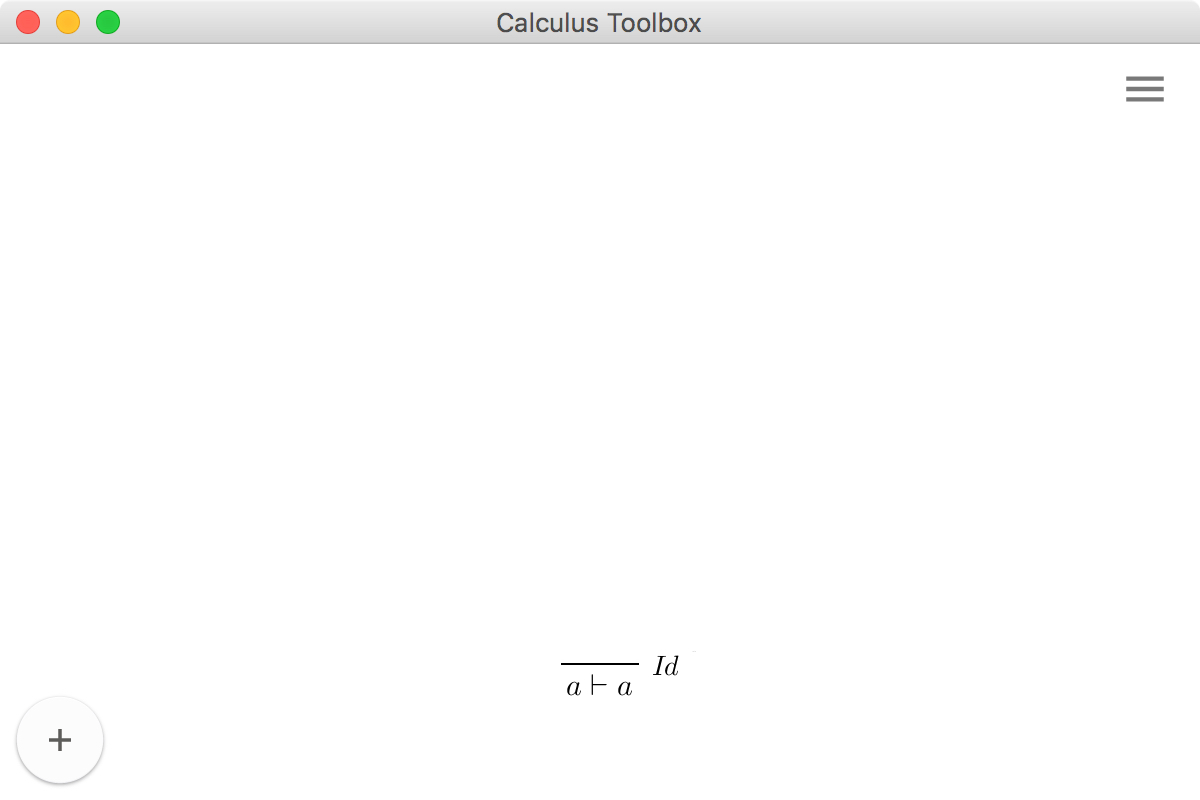
To get started, let's try proving a simple statement \(\vdash A \vee \lnot A\). As was mentioned in part one of this tutorial, to simulate the empty list on the left hand side of the turnstile (\(\vdash\)) in our formalization, we use the nullary structural connective \(I\). To enter this goal into the tool press on the button with the + sign in the bottom left corner. A bar with an input box will appear. Here, the user can input a sequent, using the ASCII notation formalized in the JSON file. The tool tries to parse the expression as the user types, turning red if the term is not valid:

If the user inputs a well-formed sequent, the bar turns green, indicating the sequent is valid and can be entered:

To create a new proof tree with the entered sequent at its root, one simply has to press Enter.

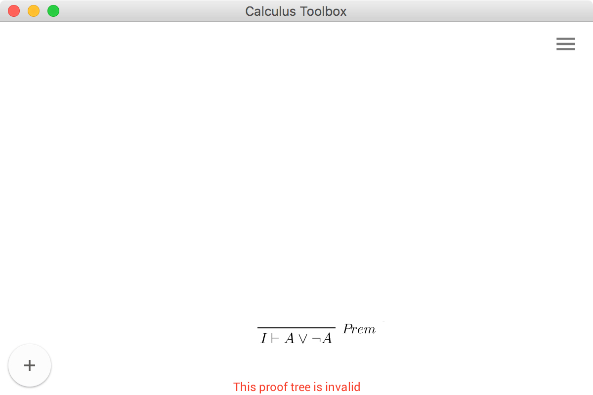
The label at the bottom warns that the current tree is not valid, meaning it contains at least one open branch. Now that we have a proof tree stub, we can start building up the proof tree.

To extend the tree, click on the sequent in the main window and select Add above from the drop down menu. The pop up that appears lists all the rules that can be applied to the current goal.

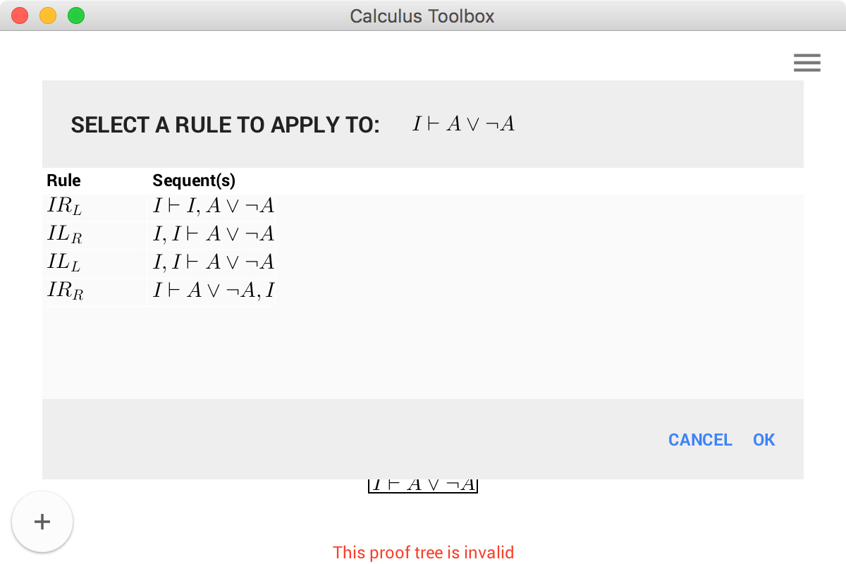
Following the proof in the wikipedia article, we first need to apply the \(CR\) rule to make two copies of the formula \(A \vee \lnot A\). Looking at the list of applicable rules, we can see that \(CR\) cannot be applied to the current goal. To see why this is the case, let's take a quick look at the rule in our description file:

"C_R" : ["?X |- ?A, ?Y", "?X |- (?A, ?A) , ?Y"]
  

Clearly, our sequent has to be of the shape \(\Gamma \vdash A, \Delta\). To remedy this, we can use the \(IR_R\) rule, introducing an \(I\) on the right side of the formula \(A \vee \lnot A\) on the right hand side of turnstile. After pressing OK the proof tree is updated with the leaf of the tree now reading \(I \vdash A \vee \lnot A, I\). Clicking on this sequent and selecting Add above now yields a much longer list of rules we can apply, including the \(CR\) rule. Applying the reverse \(IR_R\) rule after \(CR\) produces \(I \vdash A \vee \lnot A, A \vee \lnot A\). Clearly, there is some overhead due to the encoding of the calculus, as these three steps in our calculus only require a single step in the wikipedia version of the calculus. To alleviate this problem somewhat, macros come to the rescue.

What is a macro

Before we create a macro, I will try to briefly explain what a macro is in the context of our toolbox. A macro is really just a derived rule. As such, the purpose of a macro in the UI is both to allow adding derived rules to the calculus and to make the proof trees look more concise. In our case, the macro should help us hide the use of the structural rule \(IR_R\), which serves no real use in the overall progress of the proof.

By defining a macro, the tool creates a proof tree stub containing sequents with free variables. Obviously, this tree is not a valid one, as we do not allow valid sequents to contain free variables. However, the macro tree stub becomes a quasi-template that, when applied to a sequent, unifies and replaces the free variables in the macro tree with concrete terms from the given sequent. Instead of copying the macro stub into the main proof tree, the macro is stored separately, which means that the macro takes on the appearance of a derived rule.

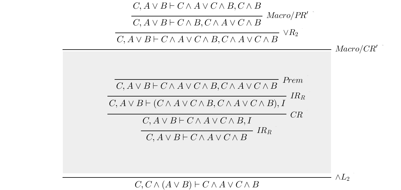
To see the tree behind the macro, we can simply click on the macro label, unfolding the hidden sub-tree:

Creating a new macro

To create a macro, we first have to build a tree that will serve as the template. The tree we want is the following:

\[\frac{\displaystyle \frac{\displaystyle \frac{\displaystyle \Gamma \vdash A , A} {\Gamma \vdash (A , A), I}} {\Gamma \vdash A, I} } {\Gamma \vdash A}\]

Here \(A\), is an arbitrary formula such as \(A \vee \lnot A\) and \(\Gamma\) is an arbitrary structure (\(I\) in our case).

We hack the toolbox slightly at this point, by building a concrete proof tree in such a way, that we can the turn it into a macro tree. We can do this by simply turning \(\Gamma \vdash A\) into X |- FA. Note that this sequent does not contain any free variables, only the atomic proposition X and FA. Prepending F as we did here will later tell the UI that this atomic proposition should be replaced by a free variable of type Formula (and X should be replaced by a free variable of type Structure).

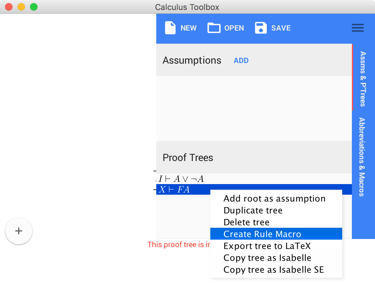
After we construct the proof tree above in the UI, we can turn it into a macro by opening the side bar by clicking on the menu button , selecting the proof tree we've just created and selecting Create Rule Macro.

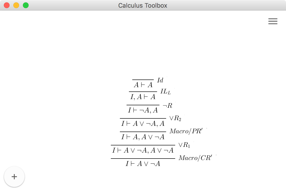
The pop up dialog shows the newly created macro, now with free variables substituted in for X and FA.

After creating the new macro rule (let's call it \(CR'\)), we can similarly create other macro rules to hide the manipulation of the \(I\)'s. We can thus create the proof for \(\vdash A \vee \lnot A\), that is almost identical to the proof in the Wikipedia article.

Saving the macros

The macros that we created in the previous section can be saved and loaded up and used in other sessions. Simply open up the side-bar menu, navigate to the Abbreviations & Macros tab and click SAVE to save the current macros. These can then be loaded up into the UI by clicking on LOAD. You can also download some pre-made macros from the Sequent calculus toolbox repository.